Observability - Integration with Spring Boot

In Coming

In our previous post, we covered the fundamental concepts of Observability.

To briefly recap:

Observability aims to understand why errors occur, and refers to the act of instrumentation — enabling even someone unfamiliar with a system’s internals to find the root cause of a problem.

The three most important pillars of Observability are:

1. Metric
2. Trace
3. Log

Therefore, when operating an application, it is critical to establish a foundation for producing data across all three pillars and forwarding that data to the appropriate Observability storage backends.

For a refresher, see the previous post: Observability - Concepts with Grafana Examples

With that review out of the way, let’s walk through how to implement Observability in a concrete Spring Boot web application.

Integration with Spring Boot

Before we dive in, here’s a quick overview of the tech stack:

• Web application: Spring Boot
• Observability framework: OpenTelemetry
• Metric storage: Prometheus
• Trace storage: Tempo
• Log storage: Loki
• Monitoring UI: Grafana
• Performance testing tool: Locust

The goal is to build a web server on top of a Spring Boot application, extract observability data (metrics, traces, logs) using the OpenTelemetry Java agent, and ship that data to the respective Observability storage backends.

The overall system flow is illustrated below:

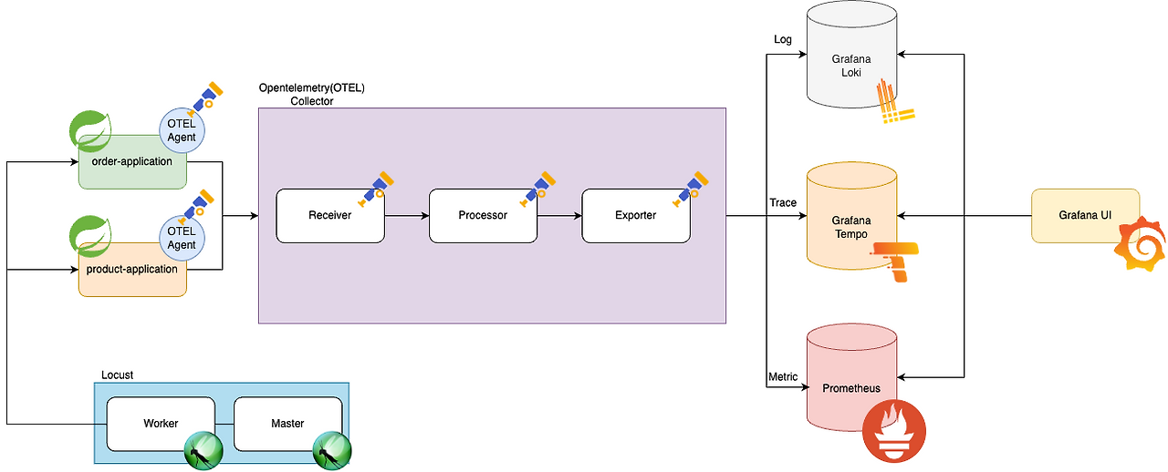
By injecting the OpenTelemetry Java agent, the application’s bytecode is modified — similar to the proxy pattern — to automatically produce and export instrumentation data.

The underlying bytecode manipulation library is ByteBuddy. A well-known project that uses it is Pinpoint.

So how do we embed the Java agent? Here’s an example using Gradle with Jib:

val agent = configurations.create("agent")

dependencies {
    // ... other libraries
    agent("io.opentelemetry.javaagent:opentelemetry-javaagent:2.7.0") // (1)
}

jib {
    from {
        image = "eclipse-temurin:21-jdk"
        platforms {
            platform {
                architecture = "arm64"
                os = "linux"
            }
        }
    }

    extraDirectories {
        paths {
            path { // (2)
                setFrom(layout.buildDirectory.dir("agent"))
                into = "/otelagent"
            }
        }
    }

    container {
        mainClass = "com.huisam.orderapplication.OrderApplicationKt"
        jvmFlags = listOf(
            "-javaagent:/otelagent/opentelemetry-javaagent.jar" // (3)
        )
    }
}

tasks.named("jibDockerBuild").configure {
    dependsOn(copyAgent)
}

Here’s what each step does:

1. Declares the OpenTelemetry agent as a downloadable dependency using a dedicated Gradle configuration.
2. During the Docker image build with Jib, copies the agent binary into the image under /otelagent.
3. Instructs the JVM to load the copied binary as a Java agent via a JVM flag.

With that, the application is fully prepared for instrumentation. The remaining setup is handled through environment variables at runtime.

Let’s look at the docker-compose.yml configuration:

services:
  order-application:
    image: order-application:0.0.1-SNAPSHOT
    container_name: order-application
    environment:
      OTEL_SERVICE_NAME: "order-application"
      OTEL_RESOURCE_ATTRIBUTES: "service=order-application,env=dev"
      OTEL_EXPORTER_OTLP_ENDPOINT: "http://collector:4317"
      OTEL_EXPORTER_OTLP_PROTOCOL: grpc
      OTEL_INSTRUMENTATION_MICROMETER_ENABLED: true
    ports:
      - "8080:8080"
    depends_on:
      - postgres-order
      - collector

  product-application:
    image: product-application:0.0.1-SNAPSHOT
    container_name: product-application
    environment:
      OTEL_SERVICE_NAME: "product-application"
      OTEL_RESOURCE_ATTRIBUTES: "service=product-application,env=dev"
      OTEL_EXPORTER_OTLP_ENDPOINT: "http://collector:4317"
      OTEL_EXPORTER_OTLP_PROTOCOL: grpc
      OTEL_INSTRUMENTATION_MICROMETER_ENABLED: true
    ports:
      - "8081:8080"
    depends_on:
      - postgres-product
      - collector

The environment variables specify the application name, the OpenTelemetry Collector endpoint, and the protocol used for data transmission.

• The OpenTelemetry Collector receives telemetry data and forwards it to the appropriate Observability storage backends according to defined pipeline policies.
• The protocol can be either https or grpc — pick one and configure accordingly.

Next, here is the OpenTelemetry Collector configuration:

receivers:
  otlp:
    protocols:
      grpc:
        endpoint: 0.0.0.0:4317
      http:
        endpoint: 0.0.0.0:4318

processors:
  batch:
    send_batch_max_size: 1000
    send_batch_size: 100
    timeout: 10s

exporters:
  prometheusremotewrite:
    endpoint: "http://prometheus:9090/api/v1/write"

  prometheus:
    endpoint: "0.0.0.0:8889"
    enable_open_metrics: true

  otlp/tempo:
    endpoint: "http://tempo:4317"
    tls:
      insecure: true

  loki:
    endpoint: "http://loki:3100/loki/api/v1/push"

service:
  pipelines:
    metrics:
      receivers: [otlp]
      processors: [batch]
      exporters: [prometheusremotewrite]
    traces:
      receivers: [otlp]
      processors: [batch]
      exporters: [otlp/tempo]
    logs:
      receivers: [otlp]
      processors: [batch]
      exporters: [loki]

This configuration batches data every 10 seconds and forwards it to Prometheus, Tempo, and Loki. Pipelines are defined to route each signal type to the correct storage backend:

• receiver: endpoint that accepts incoming telemetry data
• processor: how data is batched and at what interval
• exporter: endpoint and settings for forwarding data to a storage backend

The instrumentation pipeline is now complete. All that’s left is visualizing the data in Grafana.

Using the Correlations introduced in the previous post, let’s see how to navigate between each observability signal. The Grafana datasource configuration looks like this:

apiVersion: 1

datasources:
  - name: Prometheus
    # ...
    jsonData:
      httpMethod: GET
      exemplarTraceIdDestinations: # (1) metric -> trace
        - datasourceUid: tempo
          name: trace_id
  - name: Loki
    # ...
    jsonData:
      derivedFields: # (2) log -> trace
        - datasourceUid: tempo
          matcherRegex: '"traceid":"(\w+)"'
          url: '${__value.raw}'
          name: traceId
  - name: Tempo
    # ...
    jsonData:
      httpMethod: GET
      tracesToMetrics: # (3) trace -> metric
        datasourceUid: prometheus
        tags: [ { key: 'service.name', value: 'job' }, { key: 'method' }, { key: 'uri' }, { key: 'outcome' }, { key: 'status' }, { key: 'exception' } ]
        queries:
          - name: 'Requests'
            query: 'sum(rate(http_server_requests_seconds_count{$__tags}[10m]))'
        spanStartTimeShift: '-10m'
        spanEndTimeShift: '10m'
      serviceMap:
        datasourceUid: prometheus
      nodeGraph:
        enabled: true
      tracesToLogsV2: # (4) trace -> log
        datasourceUid: loki
        spanStartTimeShift: '-1h'
        spanEndTimeShift: '1h'
        filterByTraceID: true
        filterBySpanID: true
        tags: [ { key: 'service.name', value: 'job' } ]

Let’s take a closer look at each numbered section.

(1) Metric to Trace

Open Grafana and look at the metric panel:

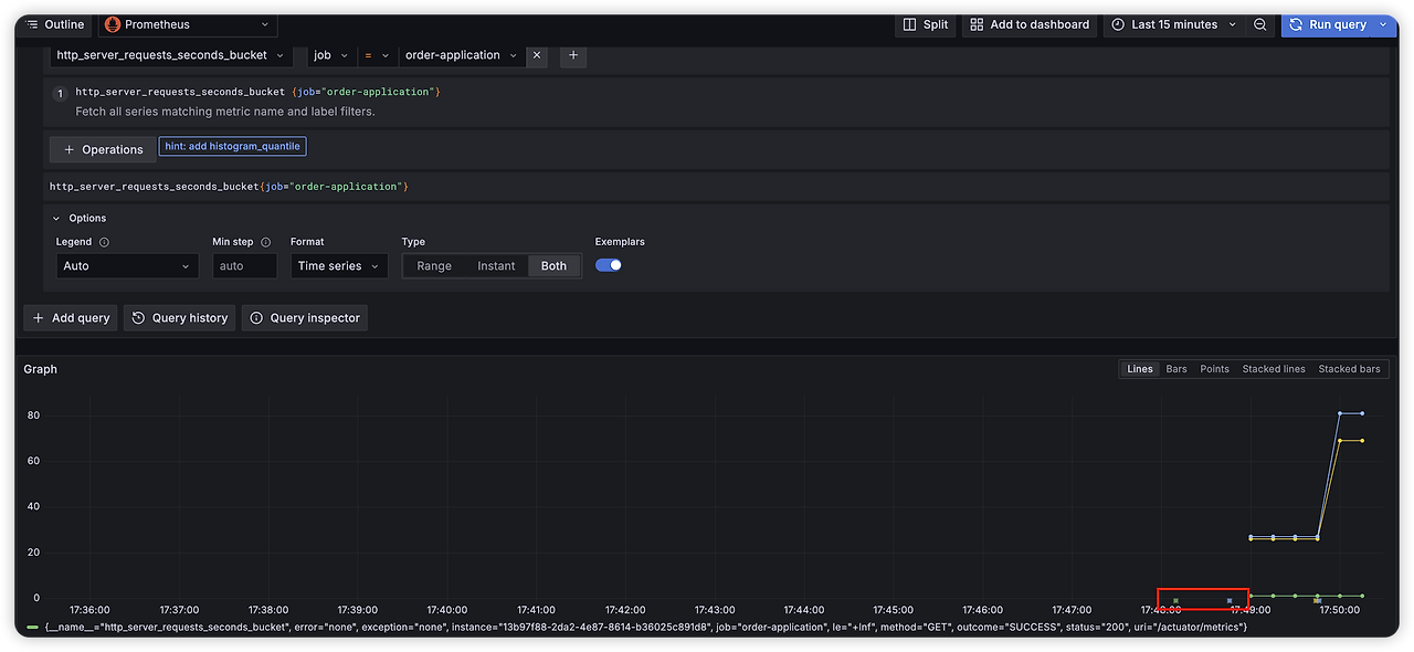
The chart is plotted on a time axis. Because sampling is performed via exemplars, you can locate a specific trace at any given point in time.

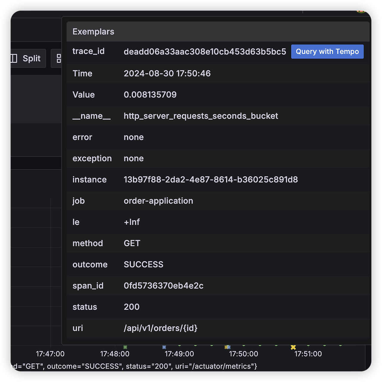
This works because of the exemplarTraceIdDestinations configuration — sampled trace representatives are embedded directly in the metric data.

From the metric view, you can navigate to a specific trace using the timestamp of a metric data point.

(2) Log to Trace

Open Grafana and look at the log panel:

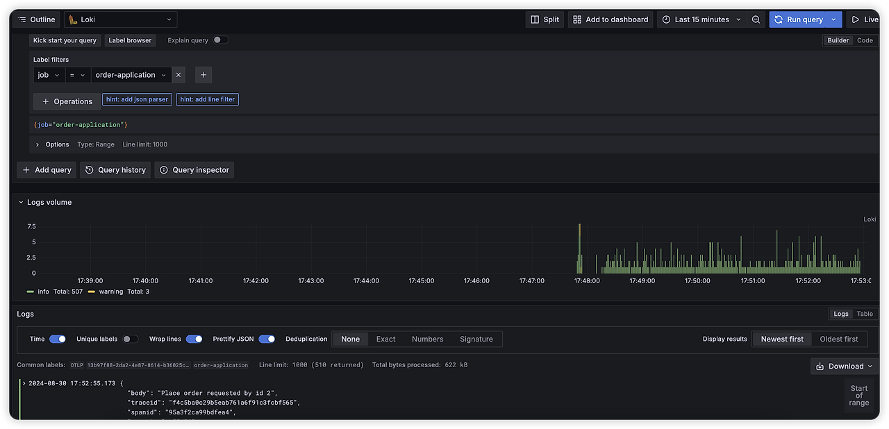
Logs are displayed in chronological order. Drilling into a log entry:

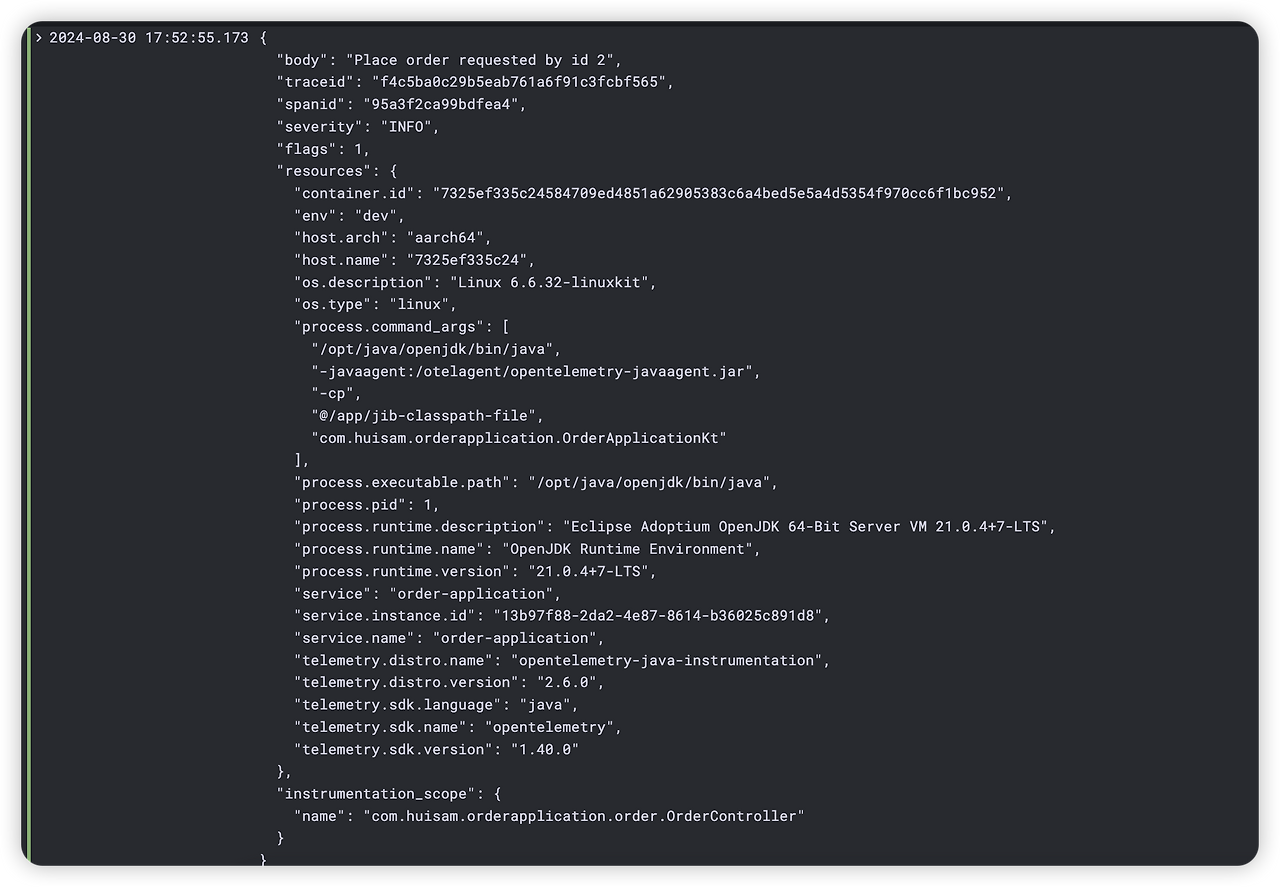
Clicking on a log entry reveals:

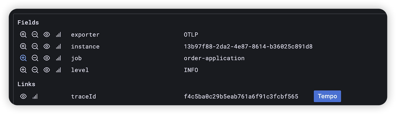
You can see the base field data along with the traceId extracted via the derivedFields configuration defined above.

This works because the application embeds trace context information (traceId, spanId) in every log record — forming the link between logs and traces.

(3) Trace to Metric

Navigate to trace data in Grafana:

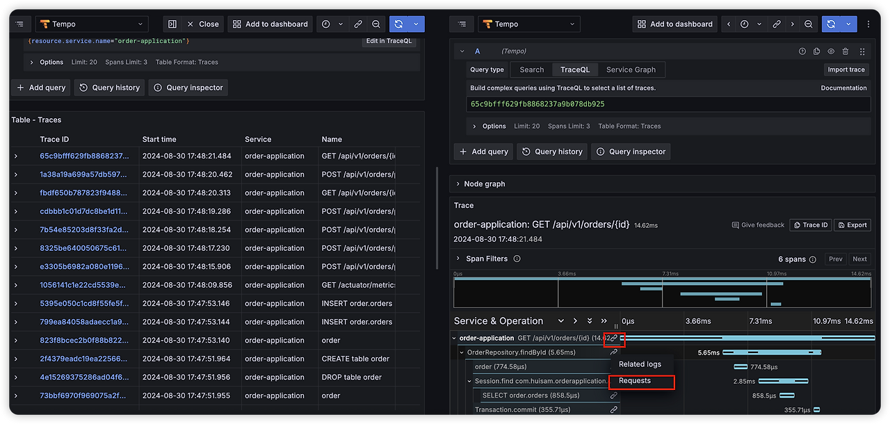
A link is available on each trace. Clicking the Requests button:

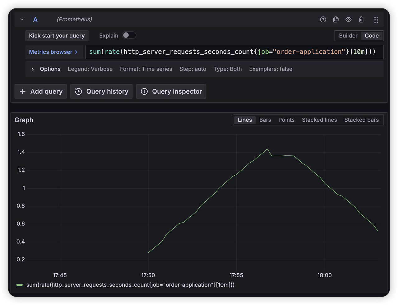
This shows request volume around the time window of that specific trace. The time window is derived from the span’s start and end time, as configured in tracesToMetrics.

(4) Trace to Log

Back in the trace view:

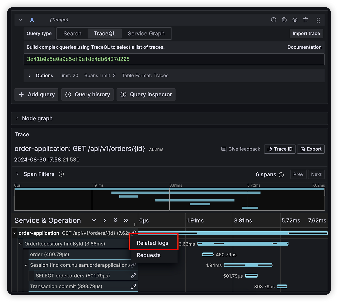
Click the Related logs button:

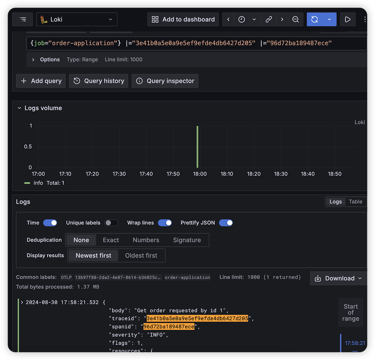
Loki is queried using the traceId and spanId, retrieving the logs for that exact span. Each bar in the trace visualization represents a single span.

If no logs were emitted during a particular span, none will be returned — that’s expected behavior.

This is configured via the tracesToLogsV2 setting.

---

And with that, Observability is fully realized in a running web application.

Not every correlation was covered here, but the key takeaway is that by connecting data through each pillar’s representative attribute, you can navigate freely across all three signals:

• Metric: scoped by time
• Trace: scoped by request
• Log: scoped by event (behavior within a specific span)

Reference

The full source code is available as open source on GitHub. If anything was unclear or you’d like to try it yourself, check it out:

GitHub - huisam/spring-observability