An easy look at the structure and principles of an LLM (feat. llama)
In Coming
Today I want to walk through the structure and the way an LLM (Large Language Model) works, in a way that is easy to follow.
The deeper you go, the more you end up explaining mathematical formulas and paper-level material, so I am not going to dive to that depth here.
Instead let’s unpack it step by step in plain language 😁
Architecture
An LLM is, at its core, a model that predicts the next token based on language and assigns a probability to it.
It is built on a neural network with billions of parameters. In the past there were models based on statistics (e.g. linear regression), but these days a neural network based approach has become the norm.
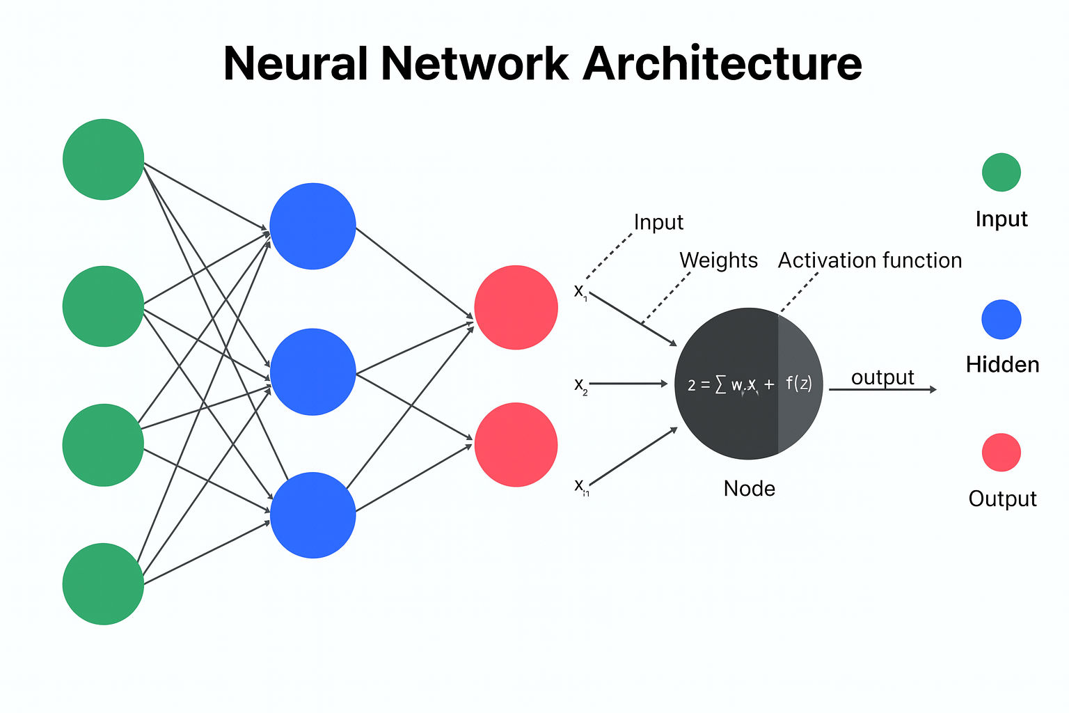
A neural network is made of layers, and each layer derives an output from the given input and its weights.
The data exchanged inside a neural network is nothing but numbers, and the language we feed into an LLM is in fact converted into numbers internally before it is passed along.
Of course a variety of formulas and principles apply along the way, but the structure of a neural network is far too complex to unfold here, so this post only touches on it briefly.
Now, if we want to get serious about the detailed structure and the working principle of an LLM, we first need to know what kind of architecture it has.
And the easiest way is always to walk through an actual LLM model as an example!
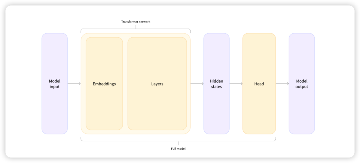
We are going to look at an architecture based on the Llama-3.2-1B model.
It is an open source model, and you can download it from Hugging Face.
1
2
3
4
5
6
7
8
9
10
11
12
13
14
15
16
17
18
19
20
21
22
23
24
25
LlamaForCausalLM(
  (model): LlamaModel(
    (embed_tokens): Embedding(128256, 2048)
    (layers): ModuleList(
      (0-15): 16 x LlamaDecoderLayer(
        (self_attn): LlamaAttention(
          (q_proj): Linear(in_features=2048, out_features=2048, bias=False)
          (k_proj): Linear(in_features=2048, out_features=512, bias=False)
          (v_proj): Linear(in_features=2048, out_features=512, bias=False)
          (o_proj): Linear(in_features=2048, out_features=2048, bias=False)
        )
        (mlp): LlamaMLP(
          (gate_proj): Linear(in_features=2048, out_features=8192, bias=False)
          (up_proj): Linear(in_features=2048, out_features=8192, bias=False)
          (down_proj): Linear(in_features=8192, out_features=2048, bias=False)
          (act_fn): SiLUActivation()
        )
        (input_layernorm): LlamaRMSNorm((2048,), eps=1e-05)
        (post_attention_layernorm): LlamaRMSNorm((2048,), eps=1e-05)
      )
    )
    (norm): LlamaRMSNorm((2048,), eps=1e-05)
    (rotary_emb): LlamaRotaryEmbedding()
  )
  (lm_head): Linear(in_features=2048, out_features=128256, bias=False)
We printed something out, but it probably still does not mean much yet, right? Let’s go through it one step at a time.
Embedding
The very first line has something called embed_tokens. I said at the beginning that this is a model that predicts tokens.
So what is a token, and what does embed mean?
First, a token is the unit you get after converting a given text into data the model can process.
In other words, the model holds a unique numeric ID per token, and internally it only passes data around based on those numeric IDs.
If the token unit is too small (1 character), the amount of data the model has to process grows exponentially and it becomes hard to capture semantic relationships.
If the unit is too large (1 word), the model has to carry an enormous vocabulary, and words with the same meaning still end up with different IDs.
For example, word and words both refer to a word, and the only difference is whether it is singular or plural.
'w','o','r','d'make it hard to capture any semantic relationship'word'and'words'carry essentially the same meaning
So as a compromise, the token unit is generally decided at the sub word level, taking similarity into account.
Let’s look at an example.
1
2
tokenizer.tokenize("Hello. I am studying about LLMs.")
# ['Hello', '.', 'ĠI', 'Ġam', 'Ġstudying', 'Ġabout', 'ĠL', 'LM', 's', '.']
You can see a single sentence being converted into the token units the model defines. What is interesting is that an abbreviation like LLMs was converted into 'L', 'LM', 's'.
Next, what about embed?
Embedding means representing the data — already converted from a token into an ID — as a vector (an N x 1 matrix).
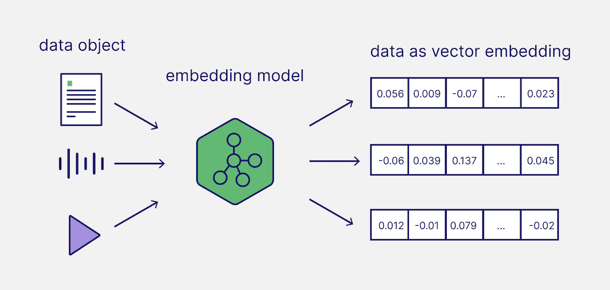
I mentioned capturing semantic relationships earlier.
That is because capturing semantic relationships matters a lot when we want to predict a token.
Think of predicting XXX in “I am XXX” versus “Smart me is XXX” — knowing the semantic relationship raises the chance of predicting XXX correctly.
So embedding is the process of turning a sentence into a high dimensional matrix.
Each token becomes a vector (an N x 1 matrix), and one sentence produces an N x N matrix holding many vectors.
Once you have that high dimensional matrix, you can compute similarity using something like the cosine function (same direction means same similarity).

Having made it through the long road of embed_token, let’s move on to the next layer.
Self Attention Layer
Now the most important part, the attention layer. From here on this is effectively the Transformer architecture.
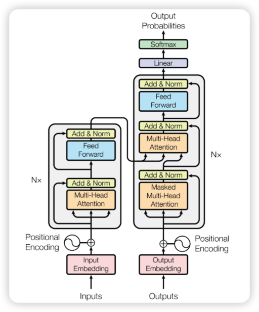
As you can see above, there are broadly two stages.
- Multi-Head Attention: figures out the context of the tokens and updates the meaning of each token (Apple could be the fruit, or the company)
- Feed forward: interprets the information the token itself carries and pulls out knowledge (the company Apple makes the iPhone)
In llama, multi head attention is composed like this.
1
2
3
4
5
6
        (self_attn): LlamaAttention(
          (q_proj): Linear(in_features=2048, out_features=2048, bias=False)
          (k_proj): Linear(in_features=2048, out_features=512, bias=False)
          (v_proj): Linear(in_features=2048, out_features=512, bias=False)
          (o_proj): Linear(in_features=2048, out_features=2048, bias=False)
        )
q, k, v, o play the following roles.
q_proj: the matrix of tokens for the Query (2048 x 2048)k_proj: the matrix of tokens for the Key (2048 x 512)v_proj: the matrix of tokens for the Value (2048 x 512)o_proj: the matrix of tokens for the Output (2048 x 2048)
The key point is Q, K and V. Each of Q, K, V is transformed by the following formula.
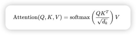
Query and Key are multiplied to check relevance, the numbers are then stabilized (the denominator), and a softmax function turns it into a probability distribution. For each probability, the Value of the other tokens in the sentence is multiplied in and everything is summed up.
In the end, this complicated chain of formulas exists to capture the meaning each individual token carries.
MLP layer
MLP (Multi Level Perceptron) means stacking perceptrons across multiple levels.
You can understand a perceptron as the most basic unit for building a neural network.
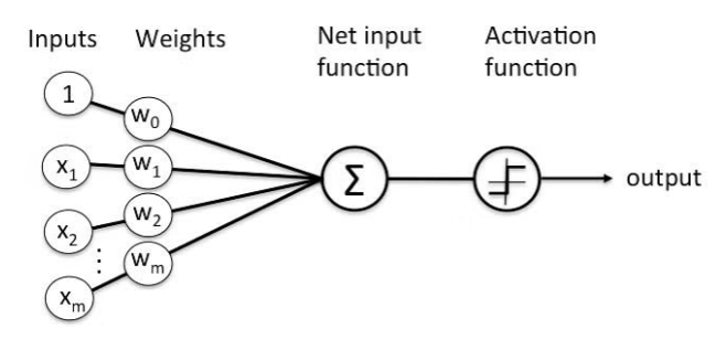
Put simply, it takes several inputs and weights and forms a single output.
So how is this actually designed in llama?
1
2
3
4
          (gate_proj): Linear(in_features=2048, out_features=8192, bias=False)
          (up_proj): Linear(in_features=2048, out_features=8192, bias=False)
          (down_proj): Linear(in_features=8192, out_features=2048, bias=False)
          (act_fn): SiLUActivation()
| Component | Description |
|---|---|
gate_proj | Expands the dimension of the input vector in order to judge how important the information is. It expands to the same dimension as up_proj. |
up_proj | Expands the dimension of the input vector. llama expands from 2048 to 8192, a 4x expansion. |
down_proj | Shrinks the widened vector back down. At this point it keeps only the important information and discards what is unnecessary (based on the gate_proj and up_proj values). |
act_fn | The activation function. It exists so the model can understand complex, abstract concepts. llama follows the SiLU function. |
As of llama 3.2, adding a gate projection to the projection layer provides the basis for feeding data through more precisely. A projection layer is simply one step for a matrix multiplication. It projects the vectors the tokens hold into an N dimensional space, so the semantic relationships those vectors carry can be inferred.
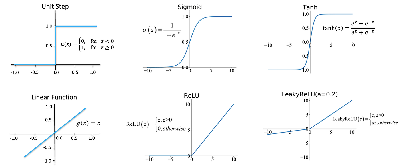
Activation functions may feel a little harder to grasp, but simply put they exist to turn a linear graph into a curved one.
To put it even more simply, they mean dropping absurd result values instead of computing with them.
As the picture shows, a linear graph has no limit on the y value, so it can expand infinitely. Once you cap the y value itself, you get a gentle curve or a shape with a very small slope, like the other graphs.
In the end, once you pass through the self attention layer and the MLP layer, predicting the next token is done.
The context of the token itself has already been captured, and the concept of the token has been expanded, so we now hold — as vector information — which token should come next.
Normalization
Looking at the principles above though, you might wonder: if things keep expanding endlessly, won’t the number of cases explode?
Normalization exists to prevent exactly that kind of excessive expansion.
1
    (norm): LlamaRMSNorm((2048,), eps=1e-05)
To explain it a bit more simply, it removes values that become too large or too small during multiplication so that everything stays within a consistent numeric range.
Once a number gets too large, the final probability distribution cannot spread evenly and ends up biased.
Normalization is a kind of stabilization step. In the llama structure there are the following normalizations.
1
2
        (input_layernorm): LlamaRMSNorm((2048,), eps=1e-05)
        (post_attention_layernorm): LlamaRMSNorm((2048,), eps=1e-05)
Placing normalization both before and after attention gives more stable results during training.
Lm head
Now that we finally have the final vector information, this vector is converted back into token language based on the token ID numbers.
1
  (lm_head): Linear(in_features=2048, out_features=128256, bias=False)
In a sense you could call it the opposite matrix of embed_token. embed_tokens was a 128,256 x 2,048 matrix, so lm_head is a 2,048 x 128,256 matrix.
So the LM head runs a matrix multiplication on the given vector and returns a score (logits) for every token the model holds.
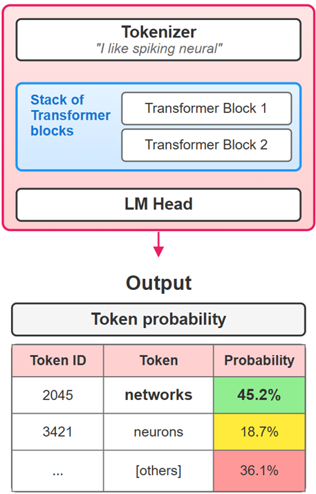
Something like this.
Parameters such as Temperature or Top_k that OpenAI or Anthropic accept are, in the end, about which multiplier is applied when turning the scores (logits) coming out of the LM head into probabilities — to flatten the probability distribution (Temperature), or to pick only the few most likely candidates (Top_k).
Conclusion
So we walked through how an LLM works, based on the llama structure, in an easy-to-follow way.
There is a lot of deep academic material behind each layer, but I tried to organize it simply without going too far in.
I hope you take this as a way to understand the basic principles and gain insight for building LLM applications.